
A Systematic, Parameter-by-Parameter Framework for Reducing IBM Cycle Time Without Compromising Container Quality — and the Calculations That Show Exactly What Each Second Saved Is Worth in Annual Production Volume
IBM machine output is determined by one number above all others: total cycle time. Every second shaved from the cycle time of a 6-cavity 100 ml PP syrup bottle line adds tens of thousands of containers to annual output without spending a cent on additional machines, tooling, or resin. Yet most IBM production lines operate 15 to 30 percent above their achievable minimum cycle time — not because of machine limitations, but because of suboptimal cooling dwell settings, conservative injection parameters, slow table index speeds, or inadequate mould cooling infrastructure.
This guide provides a systematic, engineering-based framework for IBM cycle time optimisation. It breaks total cycle time into its individual components, identifies which components are reducible and by how much, explains the physical constraints that set the true minimum for each component, and quantifies the annual output gain from each optimisation step. The goal is not to push machines to unsafe limits — it is to correctly identify and close the gap between current cycle time and the achievable minimum for each specific container, resin, and machine configuration.
1. Anatomy of an IBM Cycle: The Seven Time Components
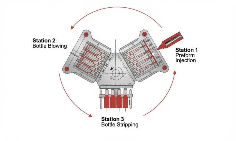
Before any optimisation can begin, total IBM cycle time must be decomposed into its constituent components. Every second of the total cycle belongs to one of seven phases, each governed by different physics and offering different degrees of optimisation potential:
| Cycle Component | Typical Duration | Governed By | Optimisation Potential |
|---|---|---|---|
| Injection fill time | 0.4 to 1.0 s | Injection speed, shot weight, resin viscosity | Low to medium |
| Hold/pack time | 0.3 to 0.8 s | Gate freeze time, hold pressure | Medium |
| Injection cooling dwell | 1.5 to 5.0 s | Neck wall thickness, mould temperature, resin Tg | HIGHEST |
| Table index time | 0.3 to 0.6 s | Machine drive speed (part of dry cycle) | LOW — machine limited |
| Blow dwell | 0.5 to 2.0 s | Body wall thickness, blow cavity cooling, resin | Medium |
| Stripping and decompression | 0.2 to 0.4 s | Machine drive speed (part of dry cycle) | LOW — machine limited |
| Screw recovery (plasticating) | 0.8 to 2.5 s | Screw speed, back pressure, shot weight | Medium (runs in parallel) |
The optimisation hierarchy: Injection cooling dwell is almost always the single largest reducible component, typically representing 30 to 50 percent of total cycle time in thin-wall small-format containers. It is governed by thermal physics — specifically how quickly the neck wall reaches a temperature below the resin’s heat deflection temperature — and responds directly to mould temperature, coolant flow rate, coolant temperature, and neck wall thickness. Reducing it by 1 to 2 seconds on a small-format line is achievable with correct infrastructure and process development. At 10 million containers per year, each second saved adds approximately 400,000 additional containers of annual output at zero additional variable cost.
2. The Output Formula: Translating Cycle Time Into Annual Bottles
The relationship between cycle time and annual output is straightforward but its implications are routinely underestimated by production managers who think of cycle time as a process variable rather than a commercial asset. The formula:
Annual Output = Cavities x (86,400 s / Cycle Time) x Uptime x Production Days
Where uptime = fraction of scheduled production time spent actually making good containers (typically 0.85 to 0.92 on a well-maintained pharmaceutical IBM line). Production days = scheduled production days per year (typically 280 to 320 for a three-shift operation with planned maintenance).
What Each Second of Cycle Time Is Worth — By Container Format
| Container / Machine Config | Cavities | Current Cycle | Annual Output | Value of 1 s Saved |
|---|---|---|---|---|
| 5 ml LDPE eye drop | 12 | 4.5 s | 63.7 M | +14.2 M / year |
| 30 ml PP oral solution | 8 | 5.5 s | 30.4 M | +5.5 M / year |
| 100 ml PP syrup bottle | 6 | 7.0 s | 19.2 M | +2.7 M / year |
| 200 ml PP cosmetic lotion | 4 | 8.0 s | 10.5 M | +1.3 M / year |
| 500 ml HDPE agrochemical | 4 | 11.0 s | 7.6 M | +0.7 M / year |
Calculations at 90% uptime, 300 production days/year. “Value of 1 s saved” = incremental annual output if cycle time reduces by exactly 1 second from the current value.
14.2 M
Extra containers per year from saving 1 second on a 12-cavity eye drop line
2.0 s
Typical achievable reduction from current to optimised cycle on most IBM lines
Zero
Additional machines, tooling, or resin needed to capture cycle time savings
30%
Typical gap between current and achievable minimum cycle on an unoptimised IBM line
3. Injection Cooling Dwell: The Largest Reducible Component
Injection cooling dwell is the time during which the core pin and parison remain stationary at Station 1 after injection fill and hold are complete, waiting for the parison neck to cool sufficiently to maintain its dimensional integrity during table index. It is the single largest component of most IBM cycle times and the primary target for optimisation.
The Physics of Neck Cooling
The minimum injection cooling dwell is reached when the hottest point in the neck wall cross-section cools below the resin’s heat deflection temperature (HDT) under 0.45 MPa load — approximately 75 to 90 degrees C for standard PP grades and 55 to 65 degrees C for LDPE. Below this temperature, the neck wall is rigid enough to survive the table index without dimensional distortion. The time required to cool from melt injection temperature (220 to 260 degrees C for PP) to HDT depends on four variables:
1. Neck Wall Thickness
Cooling time scales approximately with the square of the wall thickness. Doubling neck wall thickness quadruples the required cooling time. This is why wide-neck pharmaceutical containers (thick neck wall) have longer minimum cooling dwells than narrow-neck containers even at the same container volume.
2. Mould Temperature
The temperature differential between the melt and the mould wall drives heat extraction. A mould temperature of 8 degrees C versus 20 degrees C creates a temperature differential approximately 12 degrees C greater, reducing required cooling time by 8 to 12 percent at the neck. Chilled water supply is the most impactful infrastructure change for injection cooling dwell reduction.
3. Coolant Flow Rate
Heat extraction rate depends on the convective heat transfer coefficient at the cooling channel wall, which requires turbulent flow (Reynolds number above 4,000). A flow rate below the turbulence threshold reduces the effective cooling rate dramatically — the mould may run at the correct temperature as a bulk average while the neck zone runs hot due to insufficient flow in the neck cooling circuit specifically.
4. Melt Temperature
Every 10 degrees C reduction in melt injection temperature reduces the total heat that must be extracted from the parison, reducing cooling time approximately proportionally. Lowering PP melt temperature from 250 degrees C to 230 degrees C while maintaining complete fill reduces required injection cooling dwell by 10 to 15 percent. The constraint is minimum fill temperature — below which short shots or surface defects occur.
Minimum Cooling Dwell Estimation
A simplified estimate of minimum injection cooling dwell can be derived from Fourier’s one-dimensional heat conduction equation for a wall of half-thickness s:
tcool = (s² / (pi² x alpha)) x ln(4 x (Tmelt – Tmould) / (pi x (Teject – Tmould)))
| Resin | Thermal Diffusivity (m²/s) | Tmelt (°C) | Teject (°C) | Min Cool Dwell — 1.5 mm wall, 12°C mould |
|---|---|---|---|---|
| LDPE | 1.05 x 10⁻⁷ | 190 | 55 | ~1.3 s |
| PP homopolymer | 0.95 x 10⁻⁷ | 235 | 80 | ~1.8 s |
| PET | 1.00 x 10⁻⁷ | 275 | 90 | ~2.1 s |
| HDPE | 1.20 x 10⁻⁷ | 230 | 70 | ~1.6 s |
Values are theoretical minimums for the specified wall thickness and mould temperature. Add 0.3 to 0.5 s process safety margin to the calculated minimum when setting the validated production parameter. Actual minimum is determined by ejection quality trial at progressively reduced cooling dwell values.
The cooling dwell trial method: The correct engineering approach to minimum cooling dwell determination is a systematic step-down trial: starting from the current setting, reduce injection cooling dwell by 0.2 s increments, running 20 to 30 cycles at each step and measuring neck dimension T, E, and I at each step. The minimum acceptable cooling dwell is the shortest value at which all three neck dimensions remain within specification across all cavities. The validated production setting adds a 0.3 s safety margin to this empirical minimum. Do not use the theoretical calculation alone as the production setting — use it to define the starting search range for the empirical trial.
4. Injection Speed and Hold Time: Balancing Fill Quality Against Cycle Time

Injection Fill Time
IBM injection fill time is limited at both ends: too slow, and the melt front cools before the cavity is completely filled, producing short shots and sink marks at the parison tip; too fast, and shear heating degrades the resin at the gate, producing gate discolouration, molecular weight reduction, and additive degradation in pharmaceutical-grade containers. The optimisation target is the fastest injection speed that produces a consistently filled parison without detectable shear degradation — typically verified by UV fluorescence or solution viscosity testing in pharmaceutical applications.
For most IBM parison geometries, the optimised injection fill time falls in the range of 0.35 to 0.70 seconds. Hydraulic IBM machines typically achieve 0.5 to 0.8 s fill times due to proportional valve response lag; all-electric machines (ZQ60HE) achieve 0.3 to 0.5 s fill times due to direct servo drive response. This 0.2 to 0.3 s fill time advantage contributes to the overall dry cycle advantage of the all-electric machine.
Hold Time and V-P Switchover Optimisation
Hold time (the period during which hold pressure is applied to the melt after fill completion, packing the parison against the core pin to achieve dimensional consistency) ends when the gate freezes. The gate freeze point — determined by gate diameter, resin solidification temperature, and melt temperature — is the earliest point at which hold pressure can be removed without causing sink marks from melt flow-back through the gate.
The hold time step-down trial
Starting from current hold time, reduce by 0.1 s increments. At each step, measure parison weight and check for gate-area sink marks visually and by weight consistency. The minimum hold time is the shortest value at which parison weight is consistent within plus or minus 0.5 percent shot-to-shot and no sink marks are visible. Adding 0.1 s safety margin gives the optimised hold time. Most IBM processes run 0.2 to 0.4 s more hold time than this minimum — a significant time saving when recovered across millions of cycles.
V-P switchover position
Velocity-to-pressure switchover occurs slightly before the cavity is geometrically full, allowing the slower hold pressure to complete the last 5 to 10 percent of fill without flash. Earlier switchover (at a higher remaining volume) reduces injection fill time but increases the risk of short shot if hold pressure is insufficient. Later switchover increases fill time but is more robust. Optimise by shifting switchover position earlier in 1 percent increments of remaining stroke until the first short-shot occurrence, then back off by 2 percent for the validated setting.
5. Blow Dwell Optimisation: How Thin Is the Container Wall, Really?
Blow dwell is the time the container body spends inflated against the blow cavity walls at Station 2, cooling under blow air pressure before the cavity opens and the table indexes to stripping. Unlike injection cooling dwell — which is dominated by neck wall thickness — blow dwell is governed by body wall thickness and is typically shorter for thin-wall small-format containers.
When Blow Dwell Is the Rate-Limiting Step
Blow dwell becomes the cycle rate-limiter (rather than injection cooling dwell) in two specific situations: thick-wall large containers (HDPE 500 to 1,000 ml with body wall above 1.5 mm) and containers with very short injection cooling dwells achieved through optimised cooling infrastructure. In the second case — a well-optimised eye drop line where injection cooling dwell has been reduced to 1.5 s — blow dwell of 1.8 s may actually become the longest single component, reversing the typical hierarchy.
| Container | Body Wall | Typical Blow Dwell | Min Achievable | Rate Limiter? |
|---|---|---|---|---|
| 5 ml LDPE eye drop | 0.5 to 0.7 mm | 0.6 to 1.0 s | 0.4 s | Rarely |
| 100 ml PP syrup bottle | 0.9 to 1.2 mm | 1.0 to 1.5 s | 0.7 s | Occasionally |
| 300 ml PP lotion bottle | 1.2 to 1.6 mm | 1.5 to 2.0 s | 1.0 s | Sometimes |
| 500 ml HDPE drench bottle | 1.8 to 2.5 mm | 2.5 to 4.0 s | 1.8 s | Often |
Blow dwell optimisation uses the same step-down trial approach as injection cooling dwell. The minimum blow dwell is the shortest value at which the container body retains its dimensional shape and surface finish after ejection — confirmed by checking body diameter and height against specification at progressively reduced blow dwell values. Beryllium copper blow cavities (thermal conductivity 4x higher than H13 steel) can reduce minimum blow dwell by 25 to 40 percent at thick body walls — a significant contribution on HDPE large-format lines where blow dwell is the primary cycle limiter.
6. Dry Cycle Time: The Machine-Dependent Floor
Dry cycle time — the time required for all machine motions (injection advance, clamp close/open, table index, blow open/close, stripping) excluding all thermal dwell periods — is a fixed property of the machine model and drive technology. It cannot be reduced by process parameter optimisation; only a machine upgrade changes it. The dry cycle time defines the absolute minimum achievable cycle time for any container on a given machine, regardless of how effectively all thermal dwells are minimised.
Practical implication: A fully optimised hydraulic ZQ60 line running a thin-wall small-format container cannot achieve a total cycle time below approximately 5.5 s regardless of how aggressively cooling dwells are reduced. The same container and mould on a ZQ60HE, with equivalent cooling optimisation, achieves approximately 4.0 s total cycle. This 1.5 s difference, compounded over a 10-year machine life at 300 days per year, represents hundreds of millions of additional containers from the all-electric machine. For producers currently near the minimum achievable cycle on a hydraulic machine, the only path to further cycle reduction is machine upgrade.
7. Cooling Infrastructure: The Upstream Bottleneck Most Lines Ignore
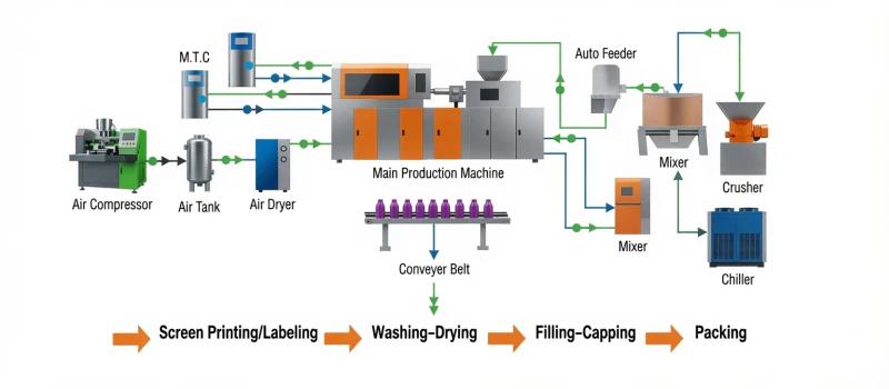
The single most common reason IBM lines fail to achieve their theoretical minimum cycle time is inadequate cooling infrastructure — specifically, mould cooling water supply that is too warm, at too low a flow rate, or poorly distributed across injection cavity cooling zones. The machine and mould may be correctly specified; the process parameters may be correctly set; but if the cooling water entering the mould is at 22 degrees C from an un-chilled facility supply rather than 10 to 14 degrees C from a dedicated chiller, the minimum achievable injection cooling dwell is 25 to 40 percent longer than the correctly-cooled case.
Cooling water temperature
A dedicated closed-loop chiller maintaining 10 to 14 degrees C supply temperature is the single highest-impact cooling infrastructure investment for IBM cycle time optimisation. The investment cost for a correctly sized chiller (typically 10 to 20 kW cooling capacity per IBM machine for small-format production) is recovered within 3 to 8 months of operation through the output increase from reduced injection cooling dwell. Below 8 degrees C, condensation on external mould surfaces becomes a contamination and safety risk in humid environments and should be avoided.
Flow rate and turbulence verification
Install a flow meter on each mould cooling circuit and verify that the flow rate is sufficient to maintain turbulent flow (Reynolds number above 4,000) in each channel. For standard 8 mm diameter injection cavity cooling channels, this requires approximately 3.5 to 5 litres per minute per circuit. If flow measurement shows laminar or transitional flow, investigate for blocked channels (scale deposits), kinked hoses, or undersized manifold fittings. Installing a separate flow indicator on the neck-zone circuit (distinct from the body-zone circuit) is specifically recommended, as the neck zone typically has the highest cooling demand and is most likely to be thermally limited.
Mould temperature measurement
Use an infrared thermometer or surface-contact thermocouple to measure injection cavity surface temperature at the neck zone during steady-state production. The cavity surface should be within 3 to 5 degrees C of the coolant supply temperature during production if channel proximity and flow rate are correct. A surface temperature 10 or more degrees C above the coolant supply temperature indicates inadequate cooling — either poor channel proximity to the cavity surface, insufficient flow rate, or fouled channels reducing heat transfer area.
Cooling circuit maintenance
Calcium scale deposits in cooling channels act as thermal insulators, reducing heat transfer rate by up to 30 percent when scale thickness reaches 0.5 mm. A descaling programme using dilute citric acid or phosphoric acid solution circulated through the cooling circuits every 6 months is standard practice for IBM lines on hard water supplies. Document coolant supply and return temperatures before and after descaling to quantify the heat transfer restoration — the temperature rise across the mould circuit (return minus supply) should decrease after descaling if scale was limiting heat transfer.
8. Melt Temperature Optimisation: Lower Is Faster (Within Limits)
Melt temperature is a frequently overlooked cycle time lever. Every 10 degrees C reduction in melt injection temperature reduces the total heat content of the parison that must be extracted during injection cooling dwell, reducing the minimum cooling dwell proportionally. For PP, a reduction from the typical 250 degrees C to 230 degrees C (a 20 degree C reduction achievable within standard process windows for most pharmaceutical-grade PP grades) reduces minimum injection cooling dwell by 12 to 18 percent — equivalent to 0.2 to 0.5 seconds on a typical syrup bottle line.
Lower melt temperature benefits
- Reduced injection cooling dwell (fewer degrees to extract)
- Reduced barrel heater energy consumption (lower setpoints)
- Reduced thermal degradation of heat-sensitive additives
- Reduced drool tendency during decompression
- Improved shot-to-shot weight consistency (lower viscosity variation)
Lower melt temperature risks
- Short shots if injection speed is not increased to compensate for higher viscosity
- Increased injection pressure demand (may approach machine limit at maximum shot weight)
- Weld mark visibility if multiple flow fronts meet at lower temperature
- Gate freeze-off occurring earlier — may reduce effective hold time if V-P settings are not adjusted
- Surface sink marks if hold time is not verified at the new temperature
Implementation approach
Reduce barrel zone setpoints by 5 to 10 degrees C in one step. Allow 20 cycles for thermal equilibrium before evaluation. Check that parison fill is complete (no short shots), hold time still produces consistent weight (check on sampling), and surface appearance is acceptable. If all pass, reduce by a further 5 degrees C and repeat. Stop at the lowest temperature that maintains complete fill, consistent weight, and acceptable surface quality. Verify neck dimensions at the optimised temperature before committing to the production parameter set.
9. Uptime and OEE: The Hidden Multiplier on Cycle Time Gains
Cycle time optimisation increases the theoretical output per available hour — but this gain is only realised if the machine is actually running during those hours. Overall Equipment Effectiveness (OEE) — the product of availability, performance, and quality rate — is the multiplier that converts theoretical cycle time improvement into actual shipped containers. An IBM line with 85 percent OEE running at the optimised cycle generates 85 percent of the theoretical output. The same line at 70 percent OEE captures only 70 percent.
OEE = Availability x Performance Rate x Quality Rate
Availability = (scheduled time – downtime) / scheduled time. Performance rate = (actual cycle time / theoretical minimum cycle time) x 100%. Quality rate = (good containers / total containers produced) x 100%. OEE values above 85% are considered world-class for IBM pharmaceutical production.
The interaction between cycle time optimisation and OEE is important: reducing cycle time by 15 percent while also reducing unplanned downtime from 12 percent to 6 percent of scheduled time produces a compounded output increase of approximately 22 percent — larger than either improvement alone. IBM lines that pursue cycle time optimisation without also addressing downtime causes (scheduled maintenance deferrals, resin change delays, cooling system failures) capture only part of their available improvement potential.
| OEE Improvement Area | Common IBM Root Causes | Typical Availability Impact |
|---|---|---|
| Unplanned downtime | Mould cooling circuit blockage, hydraulic seal failure, barrel heater burnout, cooling water chiller fault, core pin breakage | Minus 5 to 15% of scheduled time |
| Planned changeover time | Mould change, resin change, colour change, cavity count adjustment — each adding 2 to 6 hours of non-production time per event on hydraulic machines; 1 to 3 hours on ZQ60HE with recipe-stored clamping | Minus 3 to 12% of scheduled time (multi-SKU operations) |
| IPC-driven production stops | Weight out-of-specification halts requiring process re-adjustment — more frequent when cooling infrastructure is marginal and process is running close to its stable window boundary | Minus 1 to 4% of scheduled time |
10. Worked Example: From 8.0 s to 6.0 s on a 6-Cavity PP Syrup Line
The following worked example applies the full optimisation framework to a specific production scenario and shows the cumulative output gain from each step:
Baseline: 6-cavity 100 ml PP pharmaceutical syrup bottle, ZQ60 hydraulic, current cycle 8.0 s
Install dedicated chiller at 12 degrees C supply temperature
Current facility water is 22 degrees C. Chiller reduces supply to 12 degrees C, increasing temperature differential by 10 degrees C. Injection cooling dwell reduces from 3.5 s to 3.0 s. New cycle: 7.5 s. Output: 18.1 M (+1.1 M containers/year).
Verify and correct cooling circuit flow rate
Flow measurement reveals neck zone circuit at 2.1 L/min (below turbulence threshold). Manifold fitting replacement increases flow to 4.2 L/min. Neck surface temperature reduces by 6 degrees C. Cooling dwell reduces further to 2.6 s. New cycle: 7.1 s. Output: 19.1 M (+2.1 M vs baseline).
Reduce melt temperature from 250 to 232 degrees C
Step-down trial confirms complete fill and weight consistency at 232 degrees C with injection speed increased by 8%. Cooling dwell reduces to 2.3 s due to lower heat content. Hold time reduces from 0.8 s to 0.6 s after re-verification. New cycle: 6.7 s. Output: 20.3 M (+3.3 M vs baseline).
Cooling dwell step-down trial to empirical minimum
Systematic 0.2 s step-down trial with neck dimension measurement at each step establishes empirical minimum cooling dwell at 2.0 s. Validated production setting: 2.3 s (with 0.3 s safety margin). Blow dwell step-down trial reduces blow dwell from 1.5 s to 1.2 s (body wall fully rigid at this dwell at 12 degrees C coolant). New cycle: 6.2 s. Output: 21.9 M (+4.9 M vs baseline).
Final optimised cycle: 6.2 s (target 6.0 s achievable with further cooling dwell safety margin reduction after extended stability monitoring)
Annual output: 21.9 M containers (+4.9 M vs baseline, +28.8%). Investment: chiller unit + manifold fittings + process development time. No new machines, no new tooling, no additional resin, no additional labour.
11. Frequently Asked Questions
Q: How do I know if my current IBM cycle time has optimisation potential, or if it is already at the achievable minimum?
The most reliable indicator is a comparison between your current injection cooling dwell and the calculated theoretical minimum from the Fourier cooling equation for your specific neck wall thickness, resin thermal diffusivity, melt temperature, and mould temperature. If your current cooling dwell is more than 0.5 s above the theoretical minimum (accounting for the recommended 0.3 s safety margin), optimisation potential exists. A practical field check: measure the neck surface temperature with an infrared thermometer immediately after the injection cavity opens at your current cooling dwell setting. If the neck surface is below 45 degrees C (well below the HDT), your cooling dwell has safety margin that can be systematically recovered. If it is at or above 55 to 60 degrees C, you are running near the correct minimum and further reduction risks dimensional instability.
Q: Can screw recovery time limit cycle time, and how is this diagnosed?
Yes, screw recovery (the time required for the plasticating screw to recover the next shot while blowing and stripping at Stations 2 and 3) can become the cycle rate-limiter if it is longer than the combined blow dwell plus stripping time. This is diagnosed by monitoring whether the machine waits for screw recovery completion before beginning the next injection fill — a “screw not recovered” indicator on the machine’s control panel, or a measurable delay between the previous cycle’s stripping completion and the next injection advance. If screw recovery is limiting, solutions include: increasing screw speed (within shear heating limits), reducing back pressure (within shot weight consistency limits), or using a higher-MFI resin grade that plasticates faster at the same screw speed. For most small-format pharmaceutical containers, screw recovery runs in parallel and completes well within the blow dwell time — recovery limitation is more common on large-format high-weight containers.
Q: Does pharmaceutical GMP validation lock cycle time permanently once validated?
No — but changing validated cycle time parameters requires a change control process, and whether the change requires a full re-validation or an abbreviated verification depends on the magnitude of the change and its classification under the pharmaceutical producer’s quality management system. In most jurisdictions and quality systems, cycle time reduction within the previously validated process range (e.g., reducing injection cooling dwell from the validated maximum to within the validated minimum-maximum range) constitutes a routine process change verifiable by IPC sampling without full re-validation. Cycle time reduction that takes parameters outside the previously validated range requires a formal change control assessment, potentially including IQ/OQ/PQ re-execution for the affected parameters. Involve your QA team in the optimisation planning process before conducting step-down trials on a validated pharmaceutical IBM line.
Q: Will reducing injection cooling dwell affect IPC weight specifications?
Injection cooling dwell reduction, if correctly implemented at or above the empirical minimum, does not affect container weight because weight is determined by the injection fill and hold parameters — not the subsequent cooling dwell. What changes at insufficient cooling dwell is container geometry (neck dimensions T, E, I) rather than weight. Weight variation will not increase if cooling dwell is reduced to its correct minimum. However, some IBM operators confuse weight variation with cooling dwell inadequacy because both are detected at IPC sampling. The distinction: if weight is out of specification, investigate injection fill, hold pressure, and shot weight repeatability. If weight is within specification but neck dimensions are out of specification, investigate injection cooling dwell, coolant temperature, and coolant flow rate. Do not increase cooling dwell as a response to weight variation — it will not address the root cause.
12. Conclusion
IBM cycle time optimisation is one of the highest-return process engineering activities available to a container producer. The investment is primarily engineering time — systematic step-down trials, cooling infrastructure measurement, and parameter verification — with the occasional infrastructure expenditure of a chiller unit or manifold fitting upgrade. The return is a permanent increase in annual output on the same machine, tooling, and resin footprint, compounding across every production year of the machine’s 10 to 15-year life.
The framework is consistent across container formats and resin types: identify the rate-limiting cycle component (almost always injection cooling dwell), address the upstream infrastructure that constrains it (coolant temperature and flow rate), reduce melt temperature to the achievable minimum, run systematic empirical step-down trials to establish the true minimum for each component, and set validated production parameters at the empirical minimum plus a defined safety margin. The result in the worked example — a 6-cavity 100 ml PP syrup line moving from 8.0 s to 6.2 s and gaining 4.9 million additional containers per year — is representative of what a structured optimisation programme delivers.
IBM Cycle Time Optimisation — Action Checklist
Record all seven cycle time components individually. Identify which is the longest. Calculate the theoretical minimum for the injection cooling dwell using the Fourier equation for your resin and geometry.
Verify coolant supply temperature (chiller if above 15 degrees C), flow rate per circuit (flow meter, minimum turbulence Reynolds number), and cavity surface temperature (IR thermometer, maximum 5 degrees C above supply). Address deficiencies before process trials.
Lower melt temperature to achievable minimum with speed compensation. Run injection cooling dwell step-down trial in 0.2 s increments. Run blow dwell step-down trial in 0.2 s increments. Validate hold time at the new melt temperature.
Calculate the annual output gain at the optimised cycle time. If remaining gap to desired output requires further cycle reduction beyond process optimisation capability, evaluate machine upgrade from hydraulic to ZQ60HE all-electric drive.
If your IBM line is operating above its achievable minimum cycle time and you would like a structured optimisation assessment — including mould cooling audit, process parameter review, and annual output projection at optimised cycle — our applications engineering team is available to support cycle time improvement projects on ZQ-series machines. Contact us with your container specification and current cycle time for a consultation within 24 hours.
IBM Cycle Time Optimisation Consultation
Share your container specification, current cycle time, machine model, and coolant supply details. We will provide an optimisation roadmap with projected cycle reduction and annual output gain, plus a machine upgrade assessment if your current machine has reached its optimisable minimum.